Getting started¶

gmaps is a plugin for Jupyter for embedding Google Maps in your notebooks. It is designed as a data visualization tool.

To demonstrate gmaps, let’s plot the earthquake dataset, included in the package:

import gmaps
import gmaps.datasets

gmaps.configure(api_key='AI...') # Fill in with your API key

earthquake_df = gmaps.datasets.load_dataset_as_df('earthquakes')
earthquake_df.head()

The earthquake data has three columns: a latitude and longitude indicating the earthquake’s epicentre and a weight denoting the magnitude of the earthquake at that point. Let’s plot the earthquakes on a Google map:

locations = earthquake_df[['latitude', 'longitude']]
weights = earthquake_df['magnitude']
fig = gmaps.figure()
fig.add_layer(gmaps.heatmap_layer(locations, weights=weights))
fig

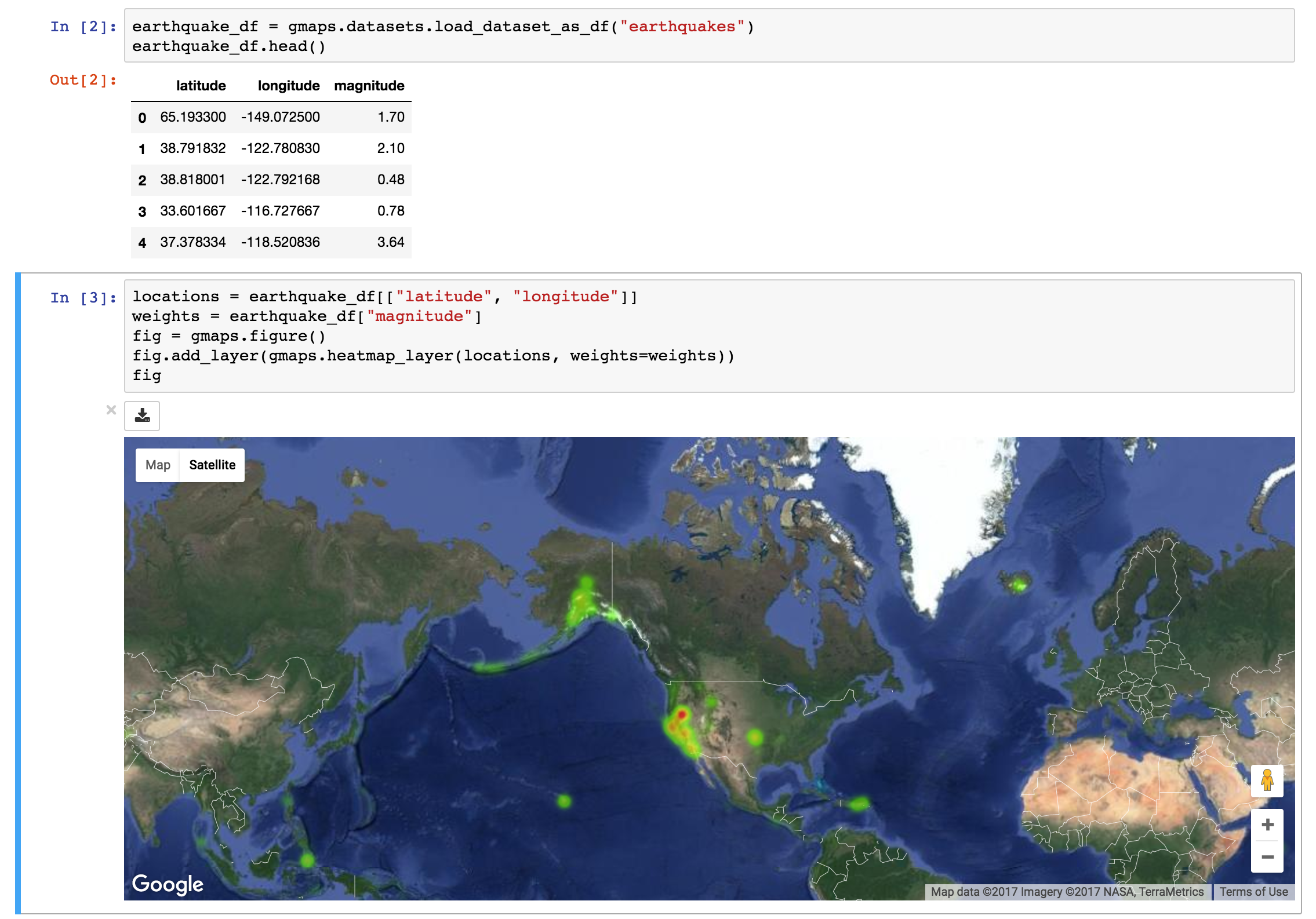
This gives you a fully-fledged Google map. You can zoom in and out, switch to satellite view and even to street view if you really want. The heatmap adjusts as you zoom in and out.

Basic concepts¶

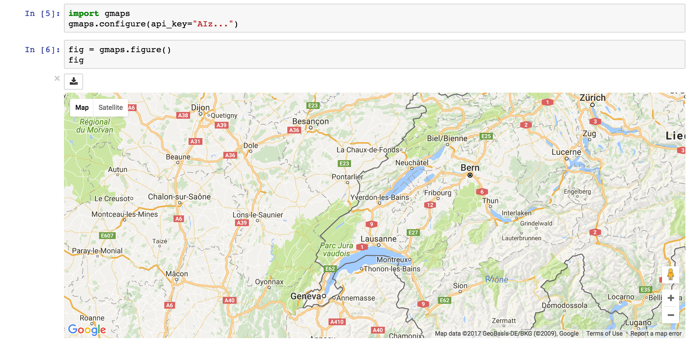
gmaps is built around the idea of adding layers to a base map. After you’ve authenticated with Google maps, you start by creating a figure, which contains a base map:

import gmaps
gmaps.configure(api_key='AI...')

fig = gmaps.figure()
fig

You then add layers on top of the base map. For instance, to add a heatmap layer:

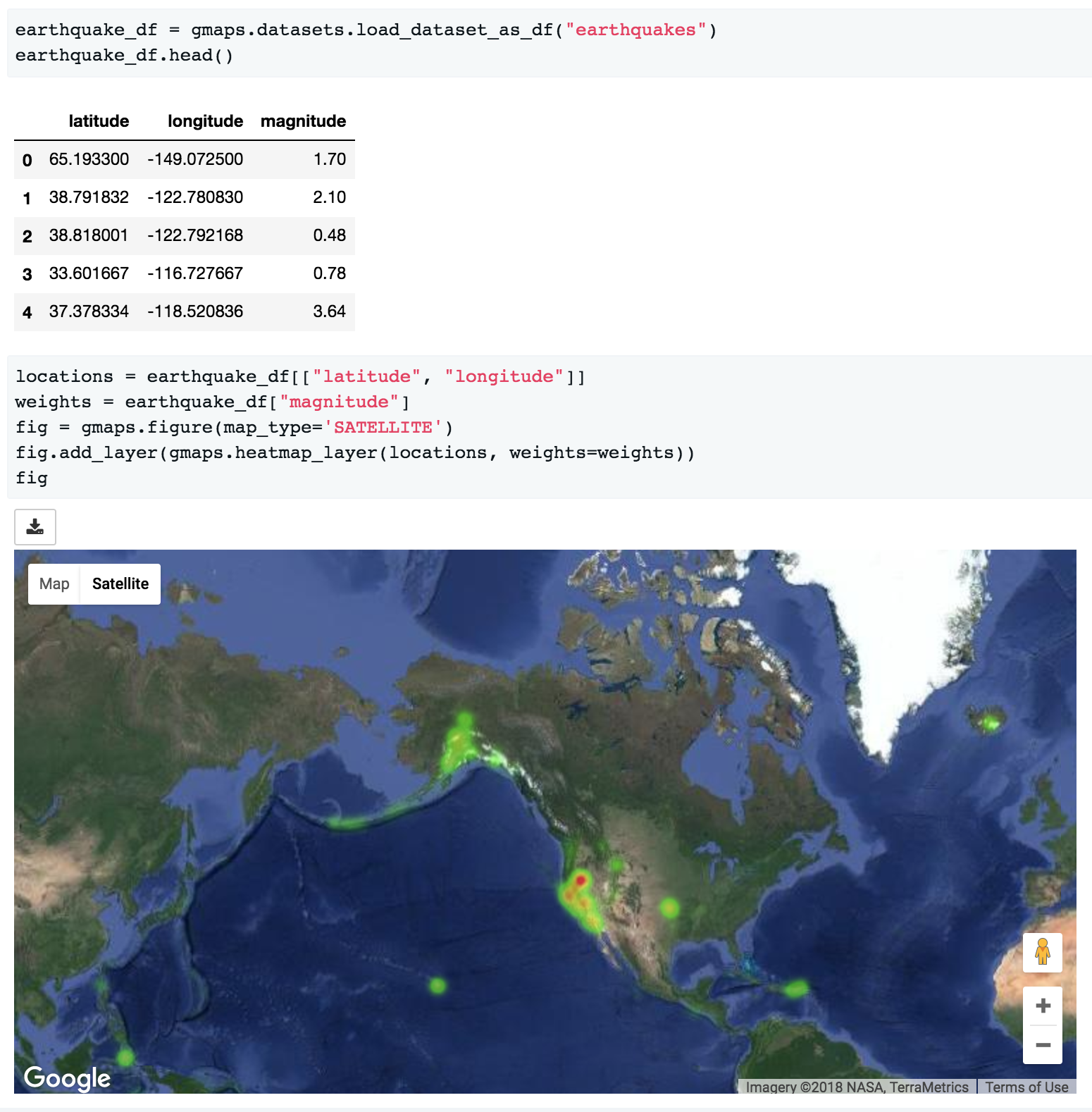
import gmaps
gmaps.configure(api_key='AI...')

fig = gmaps.figure(map_type='SATELLITE')

# generate some (latitude, longitude) pairs
locations = [(51.5, 0.1), (51.7, 0.2), (51.4, -0.2), (51.49, 0.1)]

heatmap_layer = gmaps.heatmap_layer(locations)
fig.add_layer(heatmap_layer)
fig

The locations array can either be a list of tuples, as in the example above, a numpy array of shape $N times 2$ or a dataframe with two columns.

Most attributes on the base map and the layers can be set through named arguments in the constructor or as instance attributes once the instance is created. These two constructions are thus equivalent:

heatmap_layer = gmaps.heatmap_layer(locations)
heatmap_layer.point_radius = 8

and:

heatmap_layer = gmaps.heatmap_layer(locations, point_radius=8)

The former construction is useful for modifying a map once it has been built. Any change in parameters will propagate to maps in which those layers are included.

Base maps¶

Your first action with gmaps will usually be to build a base map:

import gmaps
gmaps.configure(api_key='AI...')

gmaps.figure()

This builds an empty map. You can also set the zoom level and map center explicitly:

new_york_coordinates = (40.75, -74.00)
gmaps.figure(center=new_york_coordinates, zoom_level=12)

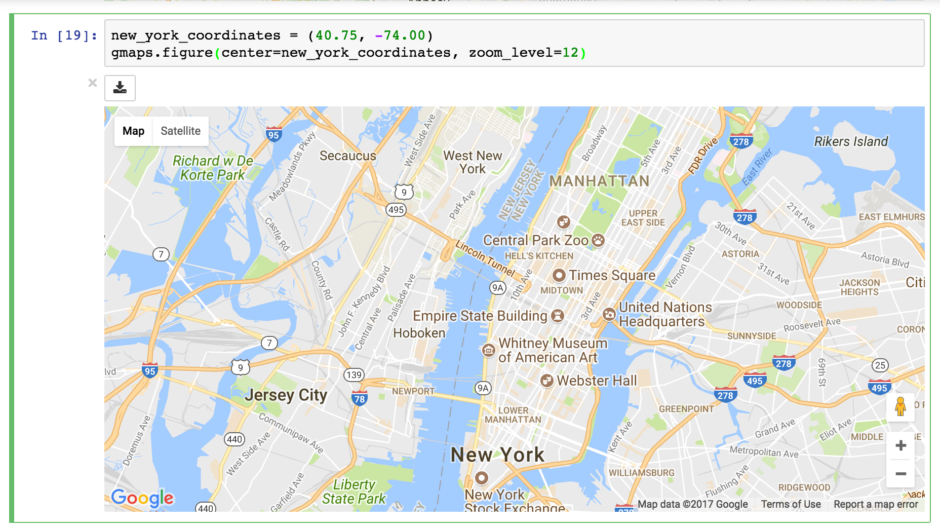
If you do not set the map zoom and center, the viewport will automatically focus on the data as you add it to the map.

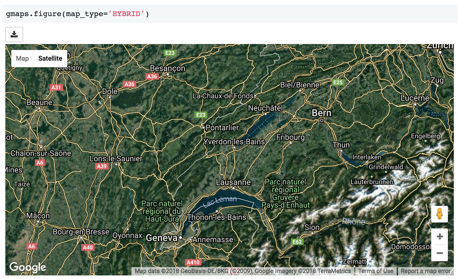
Google maps offers three different base map types. Choose the base map type by setting the map_type parameter:

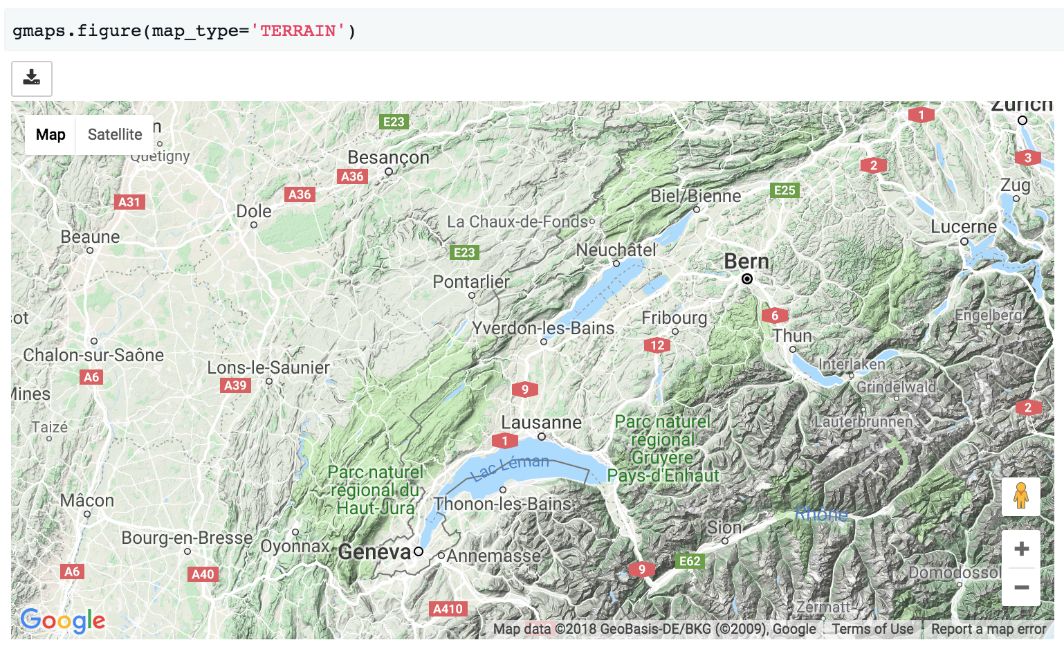
gmaps.figure(map_type='HYBRID')

gmaps.figure(map_type='TERRAIN')

There are four map types available:

'ROADMAP' is the default Google Maps style,

'SATELLITE' is a simple satellite view,

'HYBRID' is a satellite view with common features, such as roads and cities, overlaid,

'TERRAIN' is a map that emphasizes terrain features.

Customising map width, height and layout¶

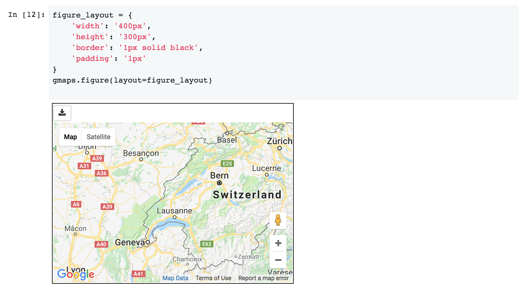
The layout of a map figure is controlled by passing a layout argument. This is a dictionary of properties controlling how the widget is displayed:

import gmaps
gmaps.configure(api_key='AI...')

figure_layout = {
    'width': '400px',
    'height': '400px',
    'border': '1px solid black',
    'padding': '1px'
}
gmaps.figure(layout=figure_layout)

The parameters that you are likely to want to tweak are:

width: controls the figure width. This should be a CSS dimension. For instance, 400px will create a figure that is 400 pixels wide, while 100% will create a figure that takes up the output cell’s entire width. The default width is 100%.

height: controls the figure height. This should be a CSS dimension. The default height is 420px.

border: Place a border around the figure. This should be a valid CSS border.

padding: Gap between the figure and the border. This should be a valid CSS padding. You can either have a single dimension (e.g. 2px), or a quadruple indicating the padding width for each side (e.g. 1px 2px 1px 2px). This is 0 by default.

margin: Gap between the border and the figure container. This should be a valid CSS margin. This is 0 by default.

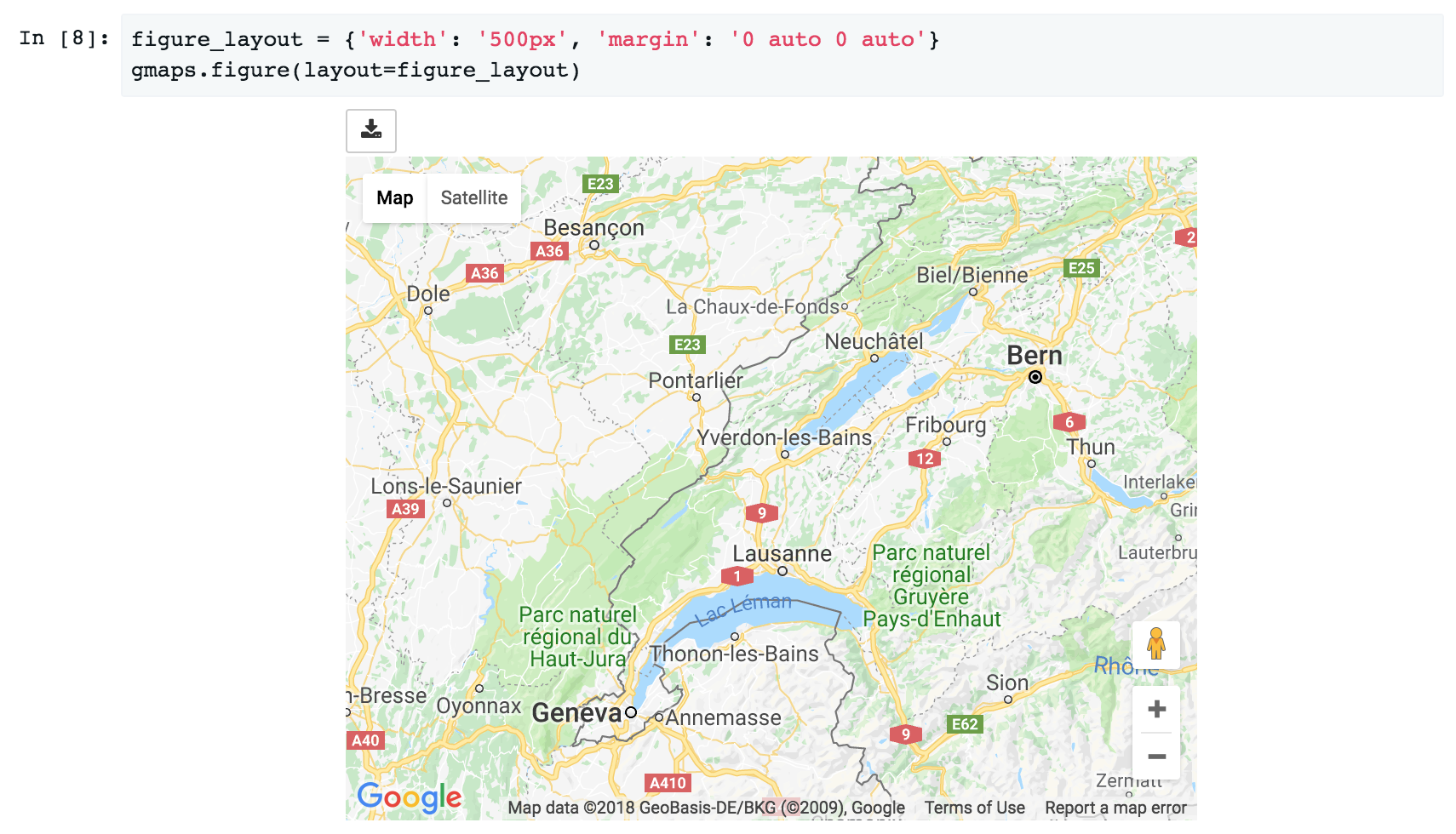
To center a map in an output cell, use a fixed width and set the left and right margins to auto:

figure_layout = {'width': '500px', 'margin': '0 auto 0 auto'}
gmaps.figure(layout=figure_layout)

Heatmaps¶

Heatmaps are a good way of getting a sense of the density and clusters of geographical events. They are a powerful tool for making sense of larger datasets. We will use a dataset recording all instances of political violence that occurred in Africa between 1997 and 2015. The dataset comes from the Armed Conflict Location and Event Data Project. This dataset contains about 110,000 rows.

import gmaps.datasets

locations = gmaps.datasets.load_dataset_as_df('acled_africa')

locations.head()
# => dataframe with 'longitude' and 'latitude' columns

We already know how to build a heatmap layer:

import gmaps
import gmaps.datasets
gmaps.configure(api_key='AI...')

locations = gmaps.datasets.load_dataset_as_df('acled_africa')
fig = gmaps.figure(map_type='HYBRID')
heatmap_layer = gmaps.heatmap_layer(locations)
fig.add_layer(heatmap_layer)
fig

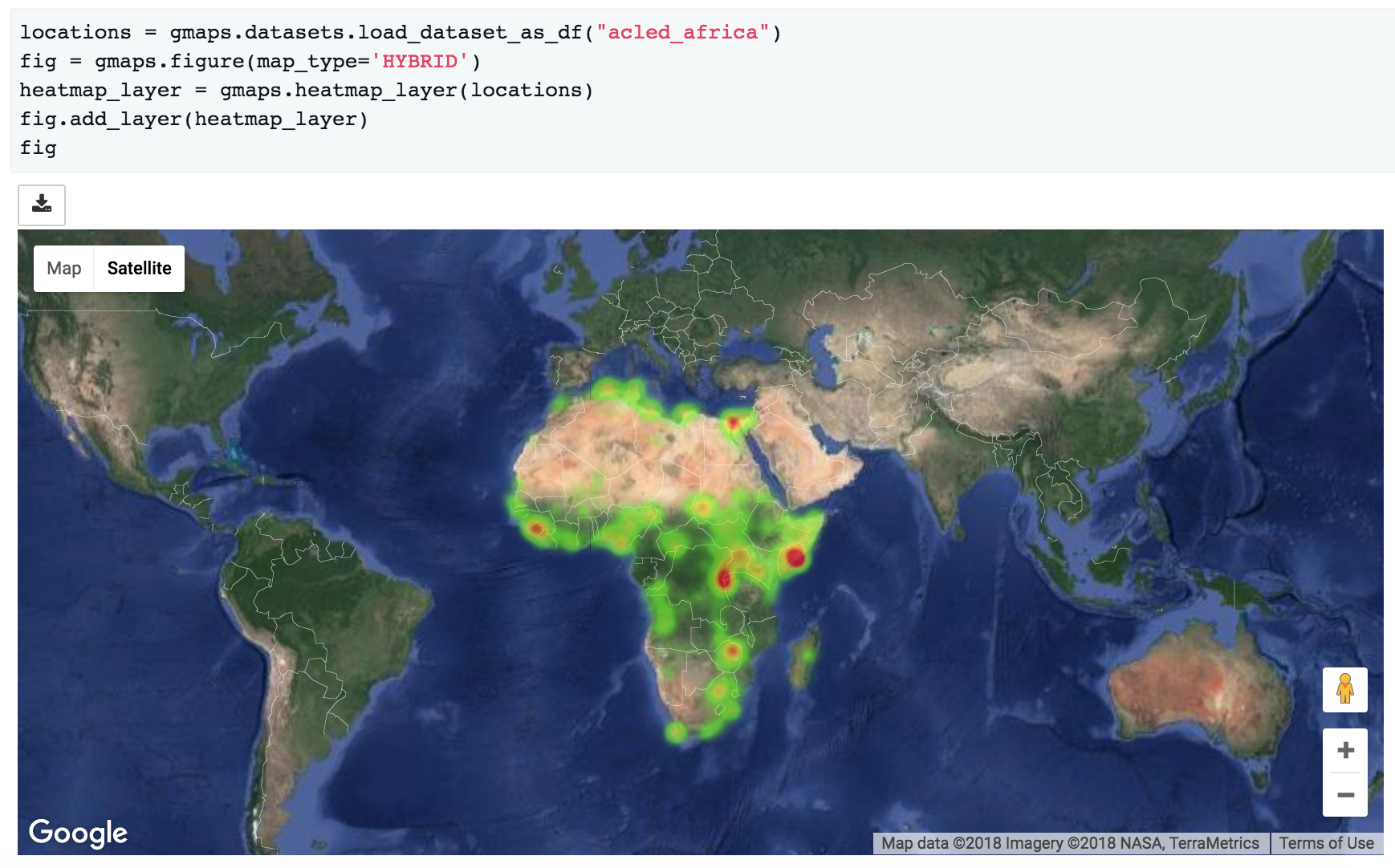
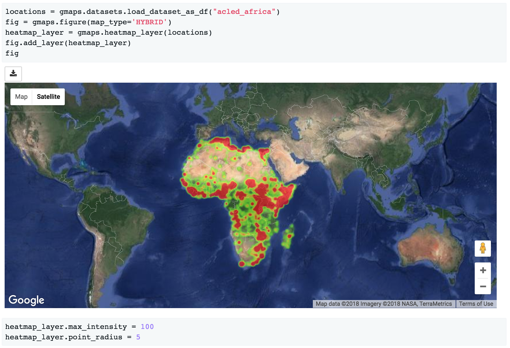
Preventing dissipation on zoom¶

If you zoom in sufficiently, you will notice that individual points disappear. You can prevent this from happening by controlling the max_intensity setting. This caps off the maximum peak intensity. It is useful if your data is strongly peaked. This settings is None by default, which implies no capping. Typically, when setting the maximum intensity, you also want to set the point_radius setting to a fairly low value. The only good way to find reasonable values for these settings is to tweak them until you have a map that you are happy with.:

heatmap_layer.max_intensity = 100
heatmap_layer.point_radius = 5

To avoid re-drawing the whole map every time you tweak these settings, you may want to set them in another noteobook cell:

Google maps also exposes a dissipating option, which is true by default. If this is true, the radius of influence of each point is tied to the zoom level: as you zoom out, a given point covers more physical kilometres. If you set it to false, the physical radius covered by each point stays fixed. Your points will therefore either be tiny at high zoom levels or large at low zoom levels.

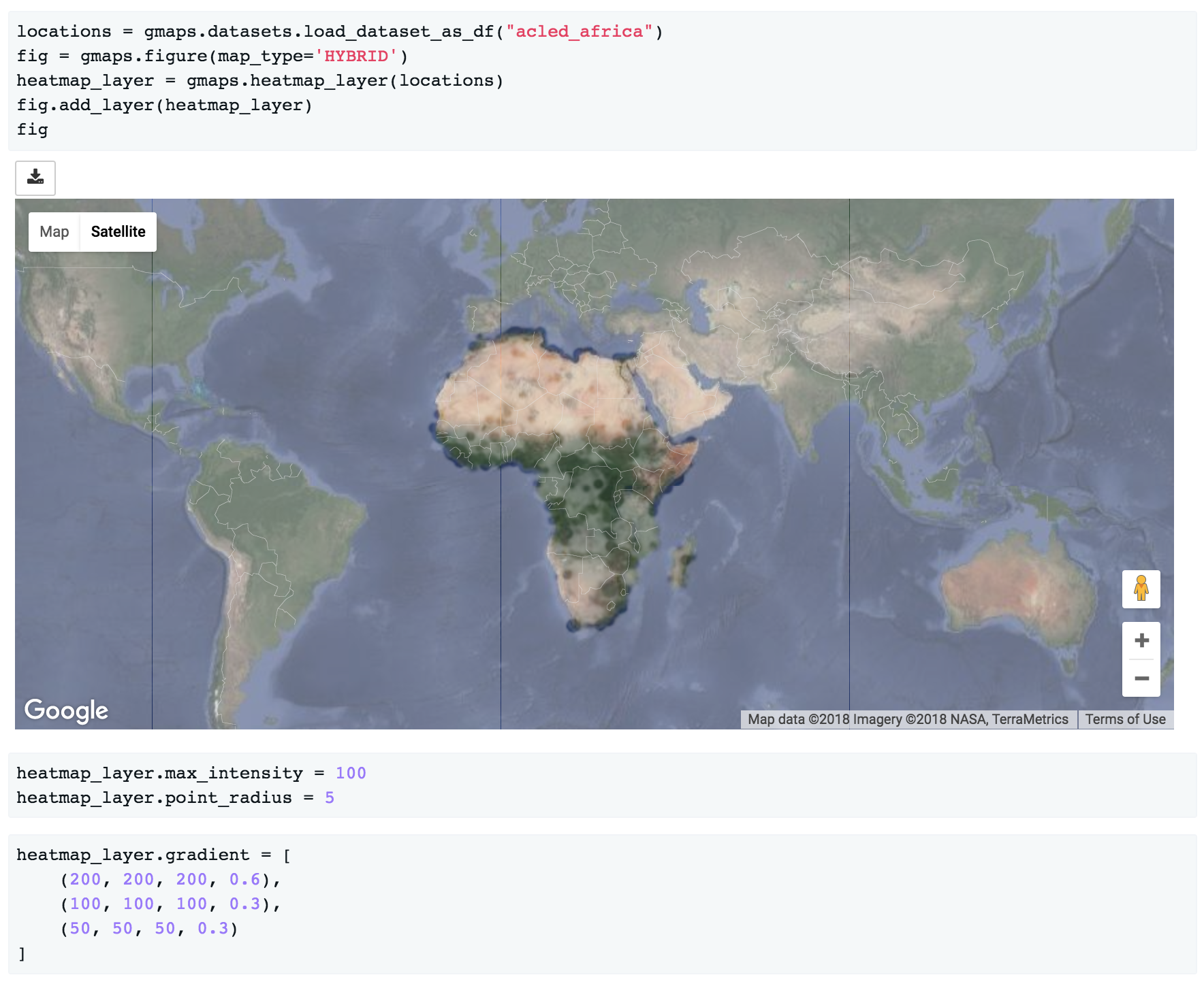
Setting the color gradient and opacity¶

You can set the color gradient of the map by passing in a list of colors. Google maps will interpolate linearly between those colors. You can represent a color as a string denoting the color (the colors allowed by this):

heatmap_layer.gradient = [
    'white',
    'silver',
    'gray'
]

If you need more flexibility, you can represent colours as an RGB triple or an RGBA quadruple:

heatmap_layer.gradient = [
    (200, 200, 200, 0.6),
    (100, 100, 100, 0.3),
    (50, 50, 50, 0.3)
]

_images/acled_africa_heatmap_gradient.png

You can also use the opacity option to set a single opacity across the entire colour gradient:

heatmap_layer.opacity = 0.0 # make the heatmap transparent

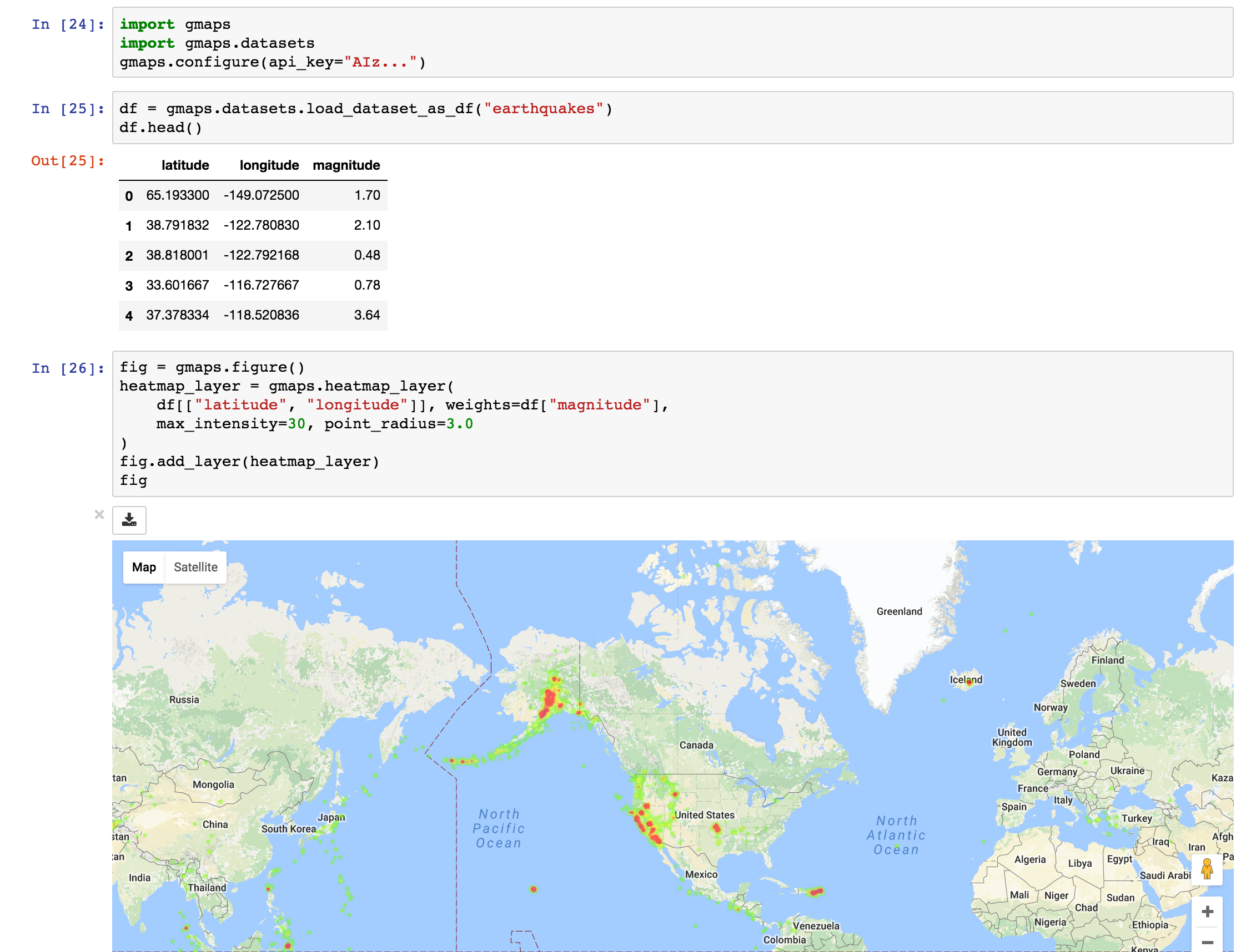
Weighted heatmaps¶

By default, heatmaps assume that every row is of equal importance. You can override this by passing weights through the weights keyword argument. The weights array is an iterable (e.g. a Python list or a Numpy array) or a single pandas series. Weights must all be positive (this is a limitation in Google maps itself).

import gmaps
import gmaps.datasets
gmaps.configure(api_key='AI...')

df = gmaps.datasets.load_dataset_as_df('earthquakes')
# dataframe with columns ('latitude', 'longitude', 'magnitude')

fig = gmaps.figure()
heatmap_layer = gmaps.heatmap_layer(
    df[['latitude', 'longitude']], weights=df['magnitude'],
    max_intensity=30, point_radius=3.0
)
fig.add_layer(heatmap_layer)
fig

Markers and symbols¶

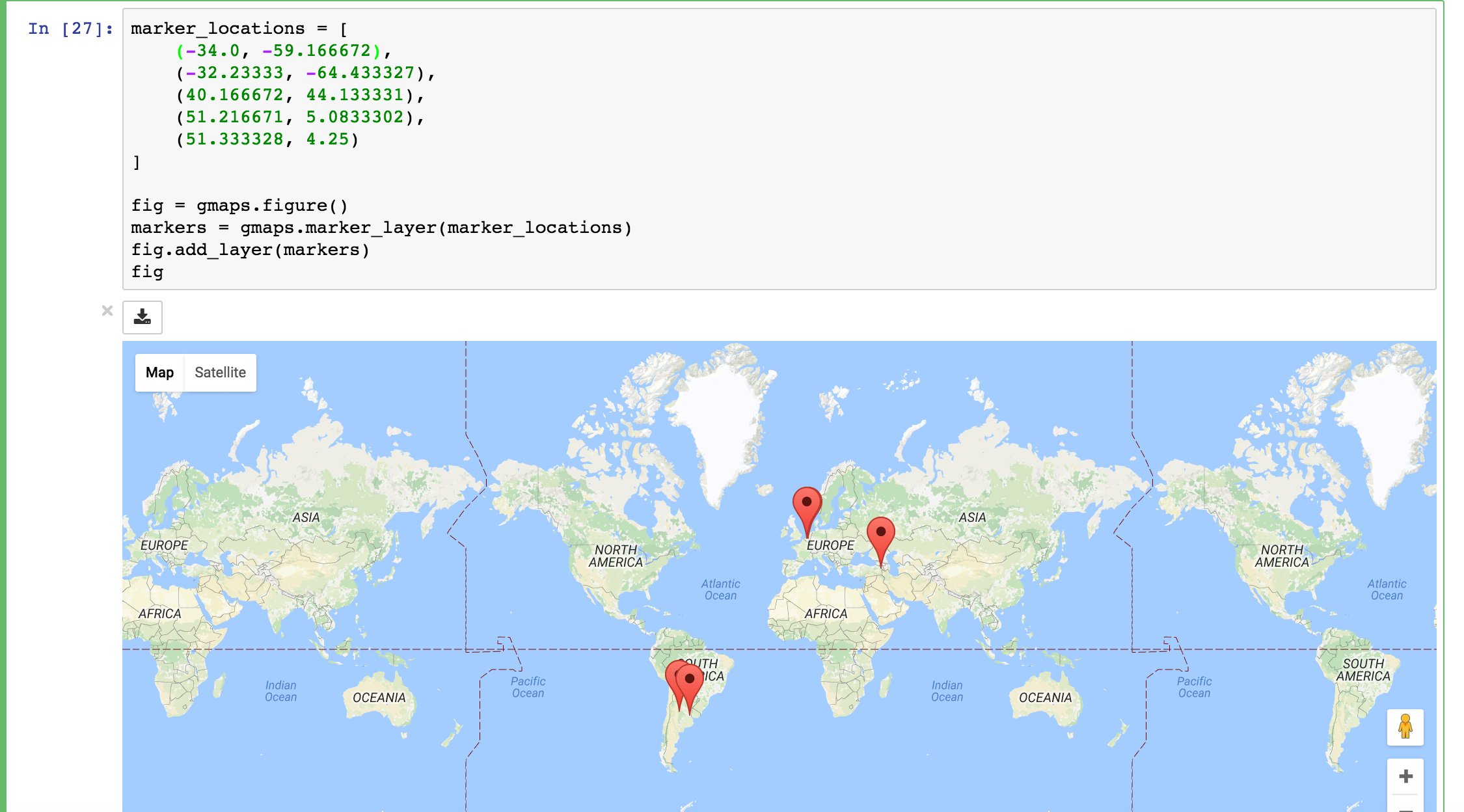
We can add a layer of markers to a Google map. Each marker represents an individual data point:

import gmaps
gmaps.configure(api_key='AI...')

marker_locations = [
    (-34.0, -59.166672),
    (-32.23333, -64.433327),
    (40.166672, 44.133331),
    (51.216671, 5.0833302),
    (51.333328, 4.25)
]

fig = gmaps.figure()
markers = gmaps.marker_layer(marker_locations)
fig.add_layer(markers)
fig

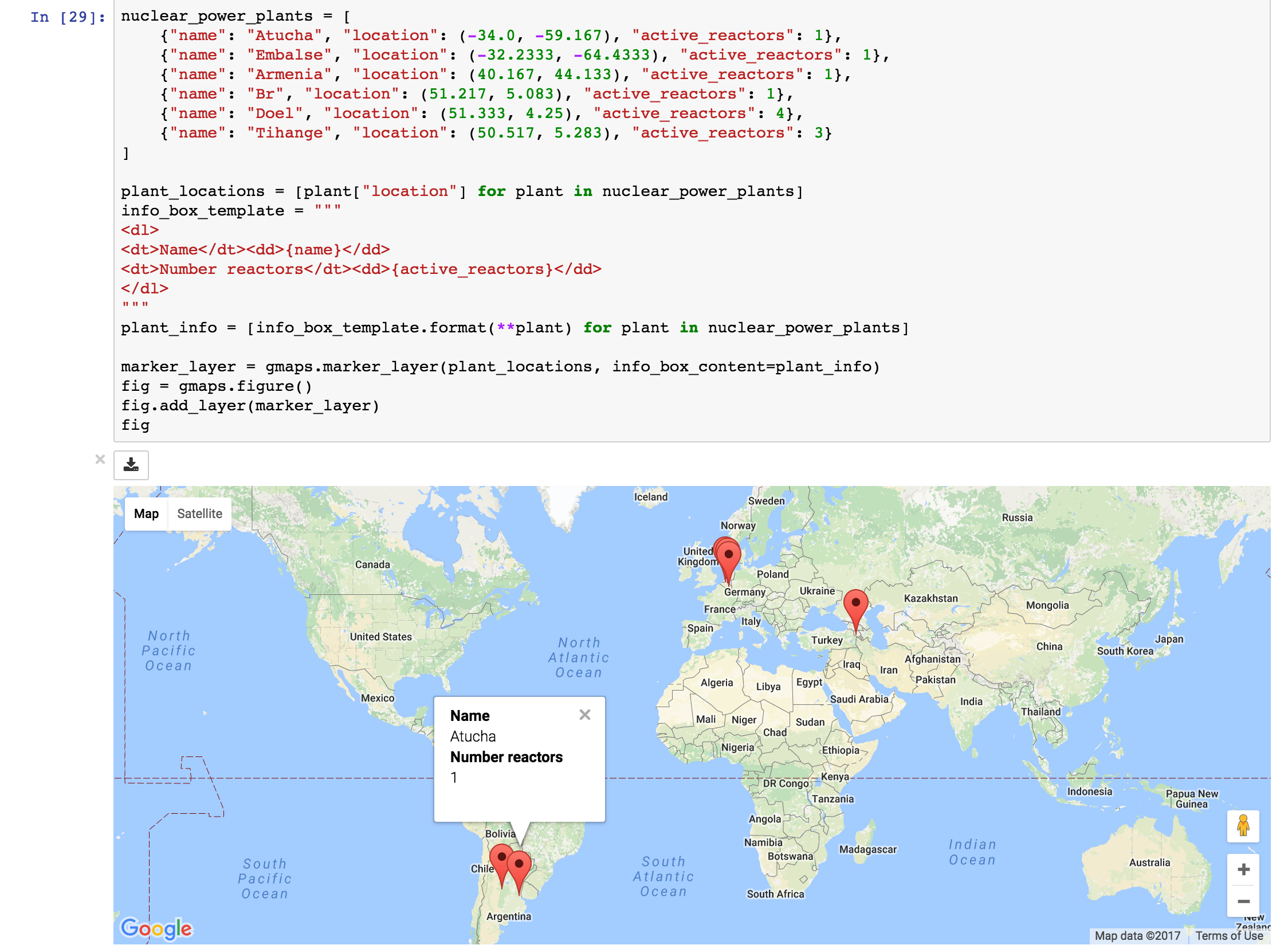
We can also attach a pop-up box to each marker. Clicking on the marker will bring up the info box. The content of the box can be either plain text or html:

import gmaps
gmaps.configure(api_key='AI...')

nuclear_power_plants = [
    {'name': 'Atucha', 'location': (-34.0, -59.167), 'active_reactors': 1},
    {'name': 'Embalse', 'location': (-32.2333, -64.4333), 'active_reactors': 1},
    {'name': 'Armenia', 'location': (40.167, 44.133), 'active_reactors': 1},
    {'name': 'Br', 'location': (51.217, 5.083), 'active_reactors': 1},
    {'name': 'Doel', 'location': (51.333, 4.25), 'active_reactors': 4},
    {'name': 'Tihange', 'location': (50.517, 5.283), 'active_reactors': 3}
]

plant_locations = [plant['location'] for plant in nuclear_power_plants]
info_box_template = """
<dl>
<dt>Name</dt><dd>{name}</dd>
<dt>Number reactors</dt><dd>{active_reactors}</dd>
</dl>
"""
plant_info = [info_box_template.format(**plant) for plant in nuclear_power_plants]

marker_layer = gmaps.marker_layer(plant_locations, info_box_content=plant_info)
fig = gmaps.figure()
fig.add_layer(marker_layer)
fig

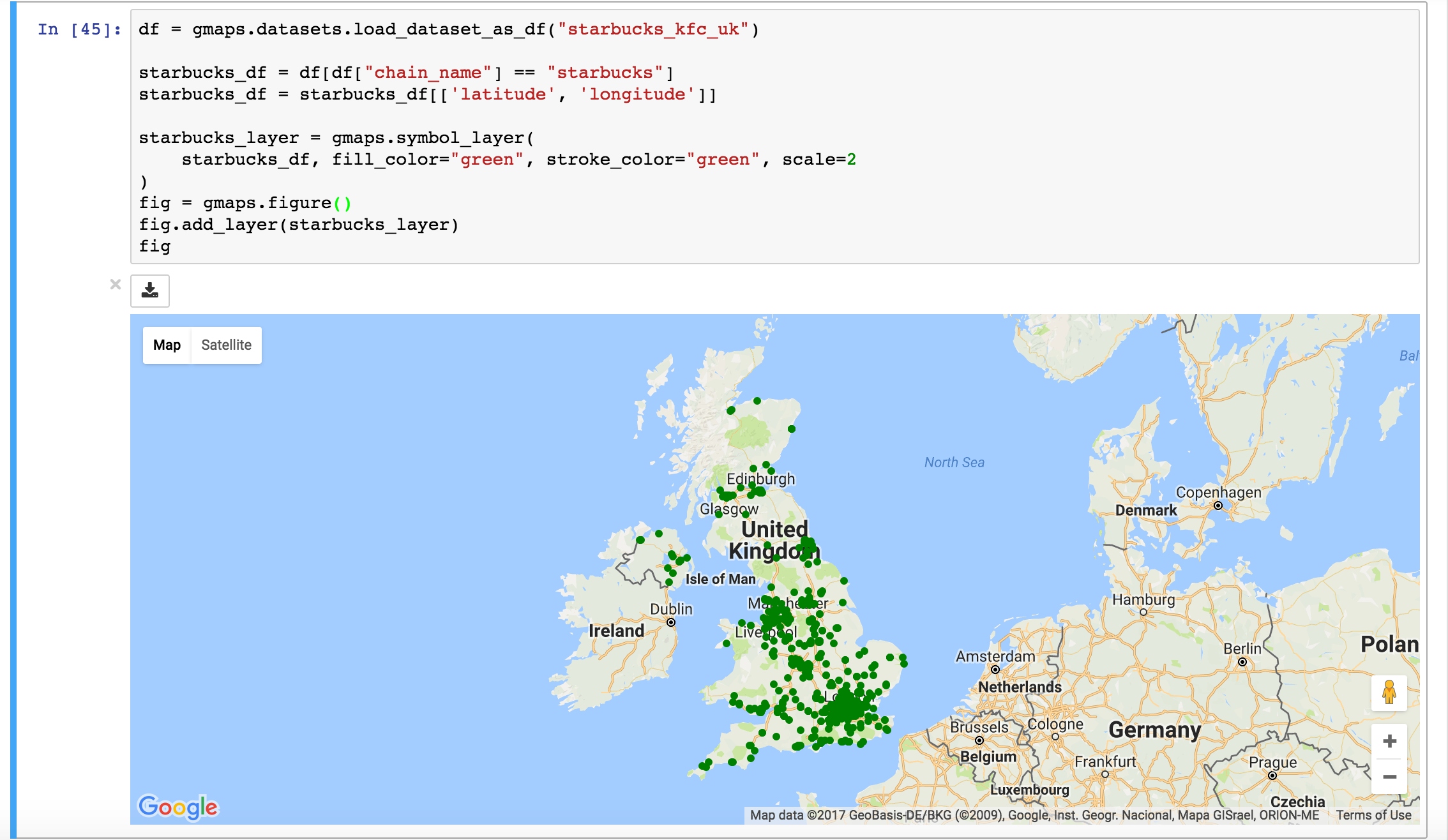
Markers are currently limited to the Google maps style drop icon. If you need to draw more complex shape on maps, use the symbol_layer function. Symbols represent each latitude, longitude pair with a circle whose colour and size you can customize. Let’s, for instance, plot the location of every Starbuck’s coffee shop in the UK:

import gmaps
import gmaps.datasets

gmaps.configure(api_key='AI...')

df = gmaps.datasets.load_dataset_as_df('starbucks_kfc_uk')

starbucks_df = df[df['chain_name'] == 'starbucks']
starbucks_df = starbucks_df[['latitude', 'longitude']]

starbucks_layer = gmaps.symbol_layer(
    starbucks_df, fill_color='green', stroke_color='green', scale=2
)
fig = gmaps.figure()
fig.add_layer(starbucks_layer)
fig

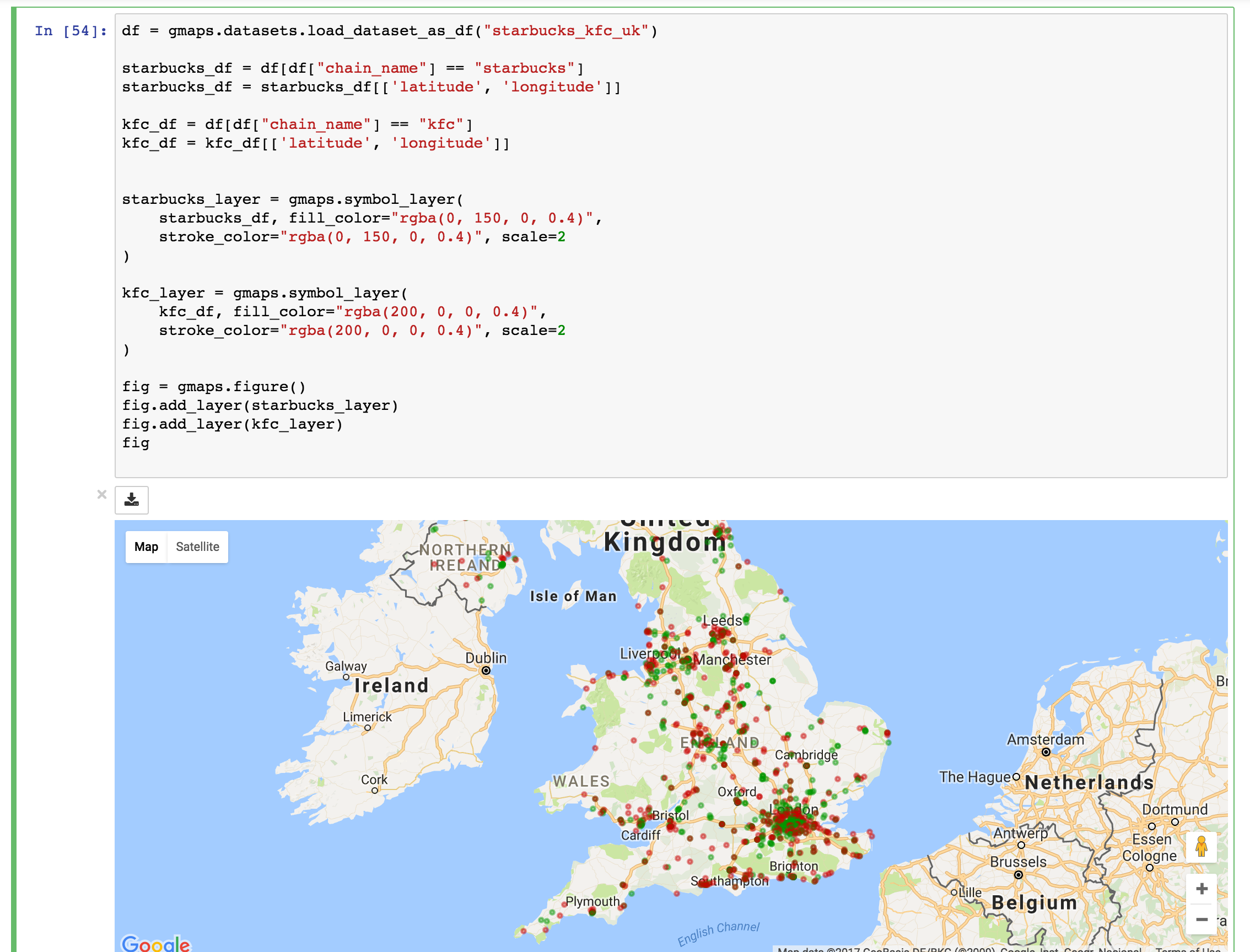
You can have several layers of markers. For instance, we can compare the locations of Starbucks coffee shops and KFC outlets in the UK by plotting both on the same map:

import gmaps
import gmaps.datasets

gmaps.configure(api_key='AI...')

df = gmaps.datasets.load_dataset_as_df('starbucks_kfc_uk')

starbucks_df = df[df['chain_name'] == 'starbucks']
starbucks_df = starbucks_df[['latitude', 'longitude']]

kfc_df = df[df['chain_name'] == 'kfc']
kfc_df = kfc_df[['latitude', 'longitude']]


starbucks_layer = gmaps.symbol_layer(
    starbucks_df, fill_color='rgba(0, 150, 0, 0.4)',
    stroke_color='rgba(0, 150, 0, 0.4)', scale=2
)

kfc_layer = gmaps.symbol_layer(
    kfc_df, fill_color='rgba(200, 0, 0, 0.4)',
    stroke_color='rgba(200, 0, 0, 0.4)', scale=2
)

fig = gmaps.figure()
fig.add_layer(starbucks_layer)
fig.add_layer(kfc_layer)
fig

Dataset size limitations¶

Google maps may become very slow if you try to represent more than a few thousand symbols or markers. If you have a larger dataset, you should either consider subsampling or use heatmaps.

GeoJSON layer¶

We can add GeoJSON to a map. This is very useful when we want to draw chloropleth maps.

You can either load data from your own GeoJSON file, or you can load one of the GeoJSON geometries bundled with gmaps. Let’s start with the latter. We will create a map of the GINI coefficient (a measure of inequality) for every country in the world.

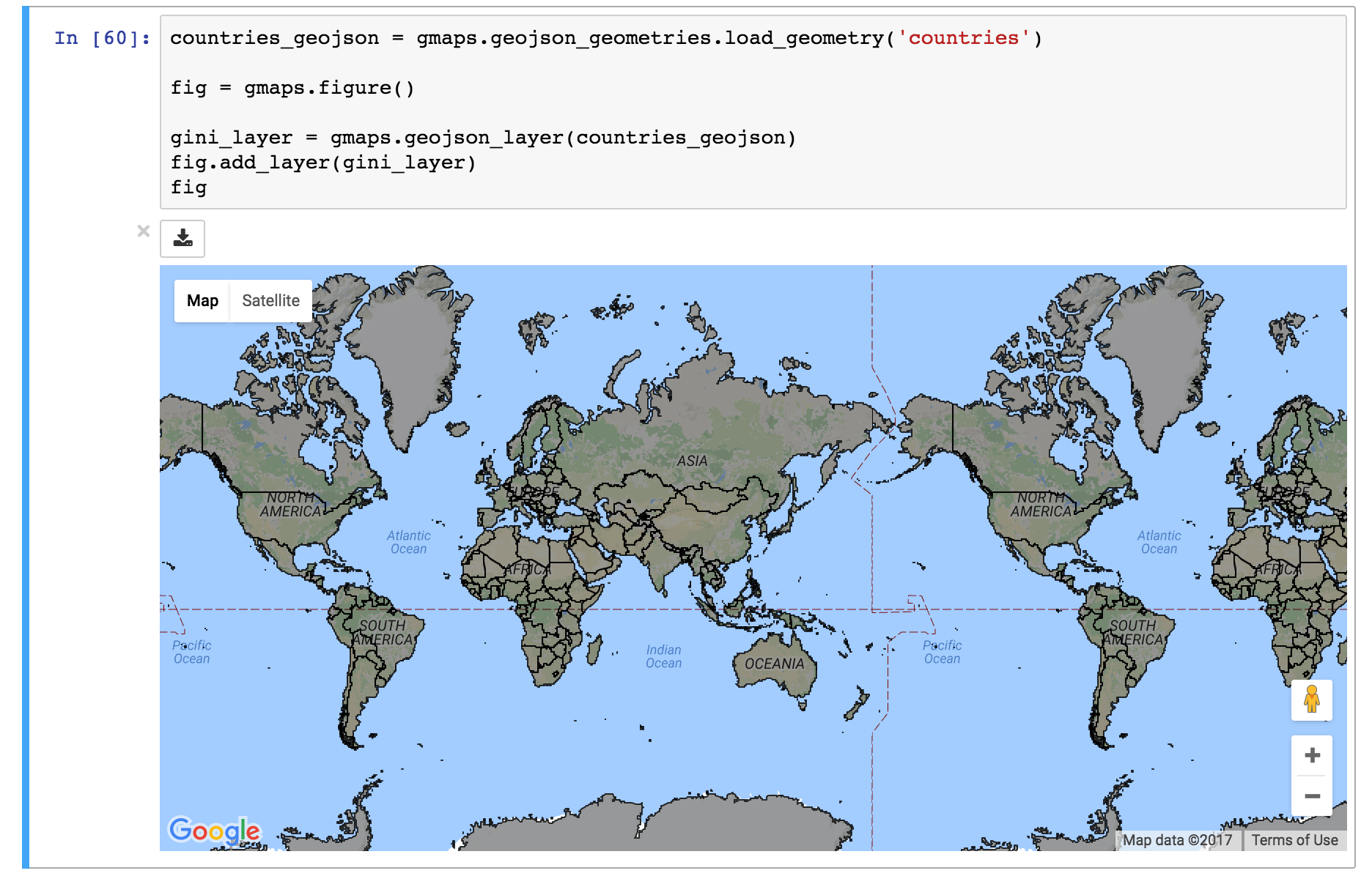
Let’s start by just plotting the raw GeoJSON:

import gmaps
import gmaps.geojson_geometries
gmaps.configure(api_key='AIza...')

countries_geojson = gmaps.geojson_geometries.load_geometry('countries')

fig = gmaps.figure()

gini_layer = gmaps.geojson_layer(countries_geojson)
fig.add_layer(gini_layer)
fig

This just plots the country boundaries on top of a Google map.

Next, we want to colour each country by a colour derived from its GINI index. We first need to map from each item in the GeoJSON document to a GINI value. GeoJSON documents are organised as a collection of features, each of which has the keys geometry and properties. For instance, for our countries:

>>> print(len(geojson['features']))
217 # corresponds to 217 distinct countries and territories
>>> print(geojson['features'][0])
{
  'type': 'Feature'
  'geometry': {'coordinates': [ ... ], 'type': 'Polygon'},
  'properties': {'ISO_A3': u'AFG', 'name': u'Afghanistan'}
}

As we can see, properties encodes meta-information about the feature, like the country name. We will use this name to look up a GINI value for that country and translate that into a colour. We can download a list of GINI coefficients for (nearly) every country using the gmaps.datasets module (you could load your own data here):

import gmaps.datasets
rows = gmaps.datasets.load_dataset('gini') # 'rows' is a list of tuples
country2gini = dict(rows) # dictionary mapping 'country' -> gini coefficient
print(country2gini['United Kingdom'])
# 32.4

We can now use the country2gini dictionary to map each country to a color. We will use a Matplotlib colormap to map from our GINI floats to a color that makes sense on a linear scale. We will use the Viridis colorscale:

from matplotlib.cm import viridis
from matplotlib.colors import to_hex

# We will need to scale the GINI values to lie between 0 and 1
min_gini = min(country2gini.values())
max_gini = max(country2gini.values())
gini_range = max_gini - min_gini

def calculate_color(gini):
    """
    Convert the GINI coefficient to a color
    """
    # make gini a number between 0 and 1
    normalized_gini = (gini - min_gini) / gini_range

    # invert gini so that high inequality gives dark color
    inverse_gini = 1.0 - normalized_gini

    # transform the gini coefficient to a matplotlib color
    mpl_color = viridis(inverse_gini)

    # transform from a matplotlib color to a valid CSS color
    gmaps_color = to_hex(mpl_color, keep_alpha=False)

    return gmaps_color

We now need to build an array of colors, one for each country, that we can pass to the GeoJSON layer. The easiest way to do this is to iterate over the array of features in the GeoJSON:

colors = []
for feature in countries_geojson['features']:
    country_name = feature['properties']['name']
    try:
        gini = country2gini[country_name]
        color = calculate_color(gini)
    except KeyError:
        # no GINI for that country: return default color
        color = (0, 0, 0, 0.3)
    colors.append(color)

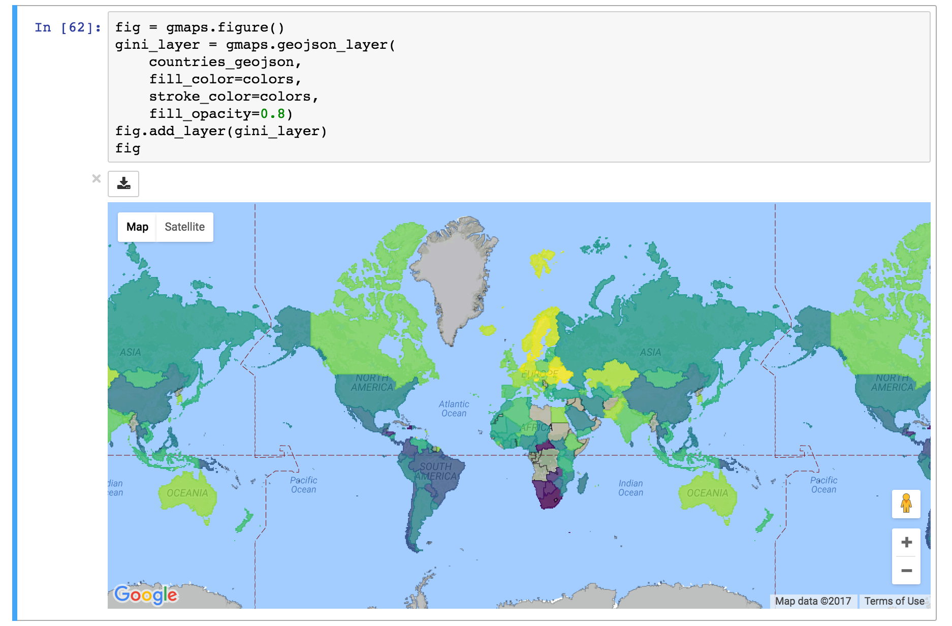
We can now pass our array of colors to the GeoJSON layer:

fig = gmaps.figure()
gini_layer = gmaps.geojson_layer(
    countries_geojson,
    fill_color=colors,
    stroke_color=colors,
    fill_opacity=0.8)
fig.add_layer(gini_layer)
fig

GeoJSON geometries bundled with Gmaps¶

Finding appropriate GeoJSON geometries can be painful. To mitigate this somewhat, gmaps comes with its own set of curated GeoJSON geometries:

>>> import gmaps.geojson_geometries
>>> gmaps.geojson_geometries.list_geometries()
['brazil-states',
'england-counties',
'us-states',
'countries',
'india-states',
'us-counties',
'countries-high-resolution']

>>> gmaps.geojson_geometries.geometry_metadata('brazil-states')
{'description': 'US county boundaries',
 'source': 'http://eric.clst.org/Stuff/USGeoJSON'}

Use the load_geometry function to get the GeoJSON object:

import gmaps
import gmaps.geojson_geometries
gmaps.configure(api_key='AIza...')

countries_geojson = gmaps.geojson_geometries.load_geometry('brazil-states')

fig = gmaps.figure()

geojson_layer = gmaps.geojson_layer(countries_geojson)
fig.add_layer(geojson_layer)
fig

New geometries would greatly enhance the usability of jupyter-gmaps. Refer to this issue on GitHub for information on how to contribute a geometry.

Loading your own GeoJSON¶

So far, we have only considered visualizing GeoJSON geometries that come with jupyter-gmaps. Most of the time, though, you will want to load your own geometry. Use the standard library json module for this:

import json
import gmaps
gmaps.configure(api_key='AIza...')

with open('my_geojson_geometry.json') as f:
    geometry = json.load(f)

fig = gmaps.figure()
geojson_layer = gmaps.geojson_layer(geometry)
fig.add_layer(geojson_layer)
fig

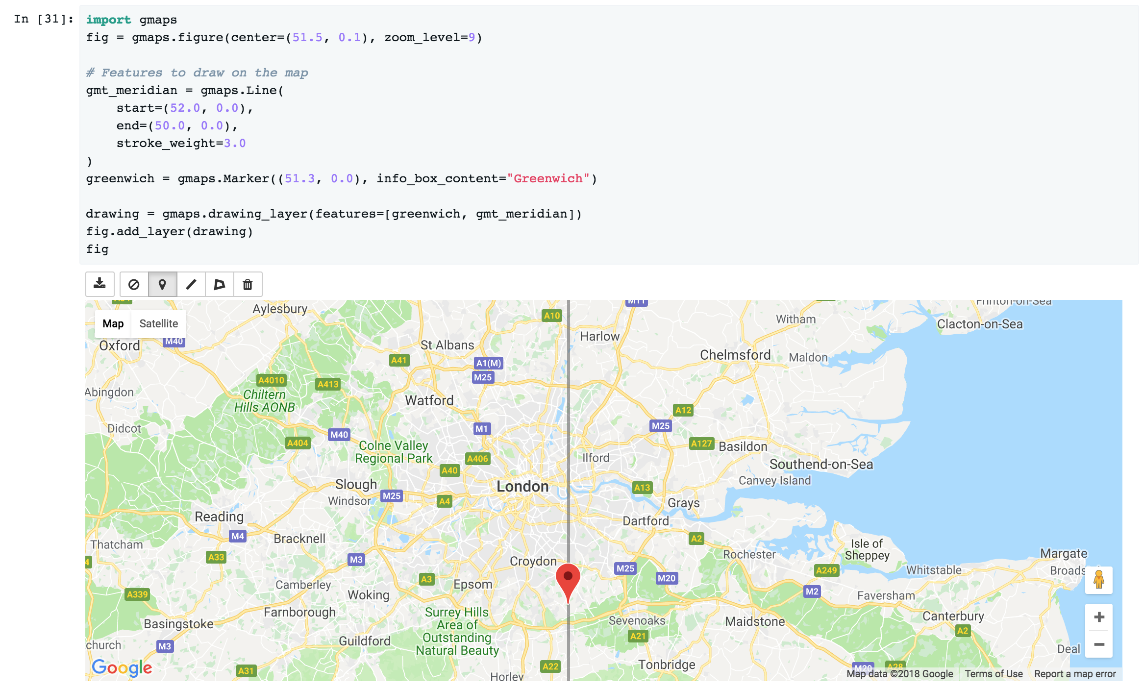
Drawing markers, lines and polygons¶

The drawing layer lets you draw complex shapes on the map. You can add markers, lines and polygons directly to maps. Let’s, for instance, draw the Greenwich meridian and add a marker on Greenwich itself:

import gmaps
gmaps.configure(api_key='AIza...')

fig = gmaps.figure(center=(51.5, 0.1), zoom_level=9)

# Features to draw on the map
gmt_meridian = gmaps.Line(
    start=(52.0, 0.0),
    end=(50.0, 0.0),
    stroke_weight=3.0
)
greenwich = gmaps.Marker((51.3, 0.0), info_box_content='Greenwich')

drawing = gmaps.drawing_layer(features=[greenwich, gmt_meridian])
fig.add_layer(drawing)
fig

Adding the drawing layer to a map displays drawing controls that lets users add arbitrary shapes to the map. This is useful if you want to react to user events (for instance, if you want to run some Python code every time the user adds a marker). This is discussed in the Reacting to user actions on the map section.

To hide the drawing controls, pass show_controls=False as argument to the drawing layer:

drawing = gmaps.drawing_layer(
    features=[greenwich, gmt_meridian],
    show_controls=False
)

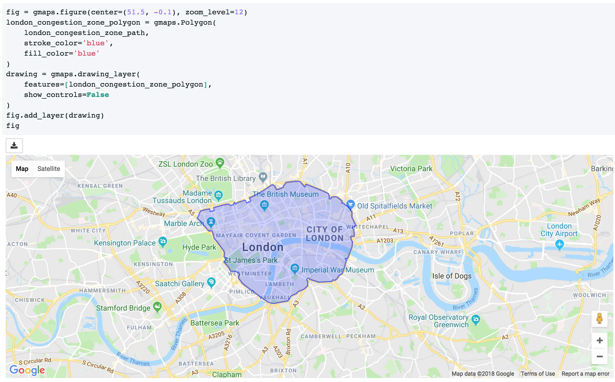
Besides lines and markers, you can also draw polygons on the map. This is useful for drawing complex shapes. For instance, we can draw the London congestion charge zone. jupyter-gmaps has a built-in dataset with the coordinates of this zone:

import gmaps
import gmaps.datasets

london_congestion_zone_path = gmaps.datasets.load_dataset('london_congestion_zone')
london_congestion_zone_path[:2]
# [(51.530318, -0.123026), (51.530078, -0.123614)]

We can draw this on the map with a gmaps.Polygon:

fig = gmaps.figure(center=(51.5, -0.1), zoom_level=12)
london_congestion_zone_polygon = gmaps.Polygon(
    london_congestion_zone_path,
    stroke_color='blue',
    fill_color='blue'
)
drawing = gmaps.drawing_layer(
    features=[london_congestion_zone_polygon],
    show_controls=False
)
fig.add_layer(drawing)
fig

We can pass an arbitrary list of (latitude, longitude) pairs to gmaps.Polygon to specify complex shapes. For details on how to style polygons, see the gmaps.Polygon API documentation.

See the API documentation for gmaps.drawing_layer() for an exhaustive list of options for the drawing layer.

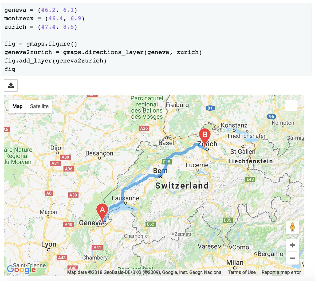
Directions layer¶

gmaps supports drawing routes based on the Google maps directions service. At the moment, this only supports directions between points denoted by latitude and longitude:

import gmaps
import gmaps.datasets
gmaps.configure(api_key='AIza...')

# Latitude-longitude pairs
geneva = (46.2, 6.1)
montreux = (46.4, 6.9)
zurich = (47.4, 8.5)

fig = gmaps.figure()
geneva2zurich = gmaps.directions_layer(geneva, zurich)
fig.add_layer(geneva2zurich)
fig

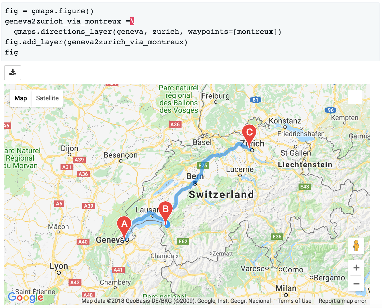
You can also pass waypoints and customise the directions request. You can pass up to 23 waypoints. Waypoints are not supported when the travel mode is 'TRANSIT' (this is a limitation of the Google Maps directions service):

fig = gmaps.figure()
geneva2zurich_via_montreux = gmaps.directions_layer(
        geneva, zurich, waypoints=[montreux],
        travel_mode='BICYCLING')
fig.add_layer(geneva2zurich_via_montreux)
fig

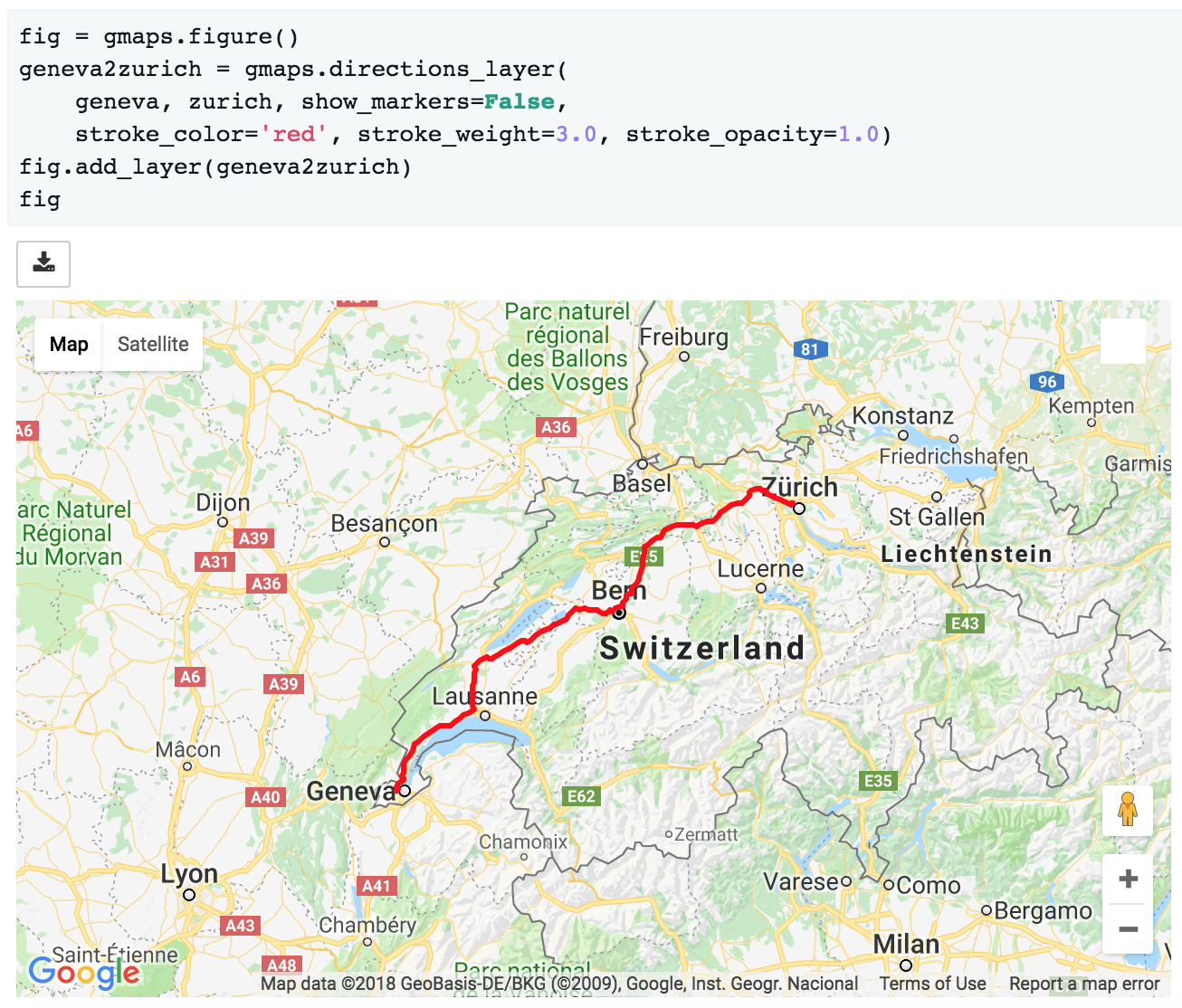
You can customise how directions are rendered on the map:

fig = gmaps.figure()
geneva2zurich = gmaps.directions_layer(
    geneva, zurich, show_markers=False,
    stroke_color='red', stroke_weight=3.0, stroke_opacity=1.0)
fig.add_layer(geneva2zurich)
fig

The full list of options is given as part of the documentation for the gmaps.directions_layer().

Updating options on the layer object will update the map. This lets you use the directions layer as part of a larger widget application. See the app tutorial for details.

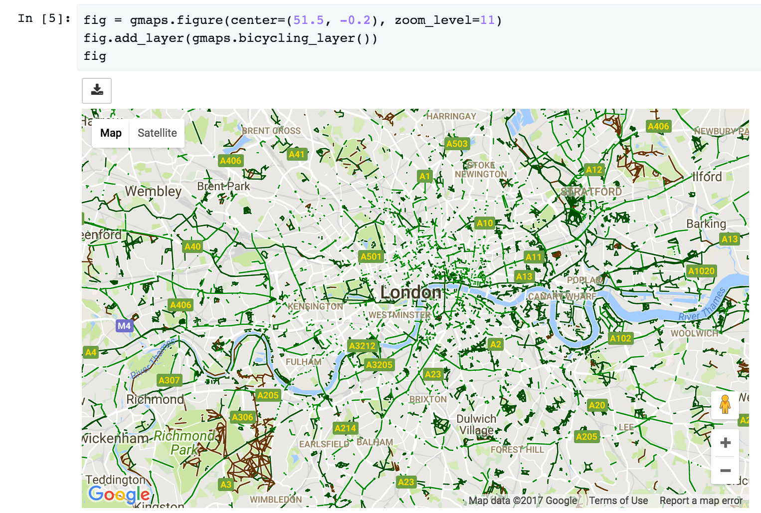
Bicycling, transit and traffic layers¶

You can add bicycling, transit and traffic information to a base map. For instance, use gmaps.bicycling_layer() to draw cycle lanes. This will also change the style of the base layer to de-emphasize streets which are not cycle-friendly.

import gmaps
gmaps.configure(api_key='AI...')

# Map centered on London
fig = gmaps.figure(center=(51.5, -0.2), zoom_level=11)
fig.add_layer(gmaps.bicycling_layer())
fig

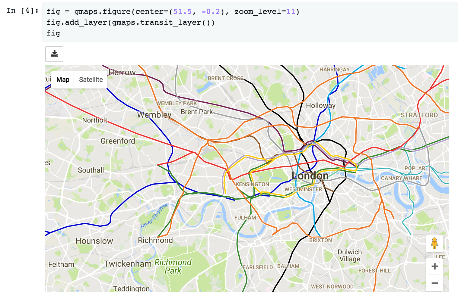
Similarly, the transit layer, available as gmaps.transit_layer(), adds information about public transport, where available.

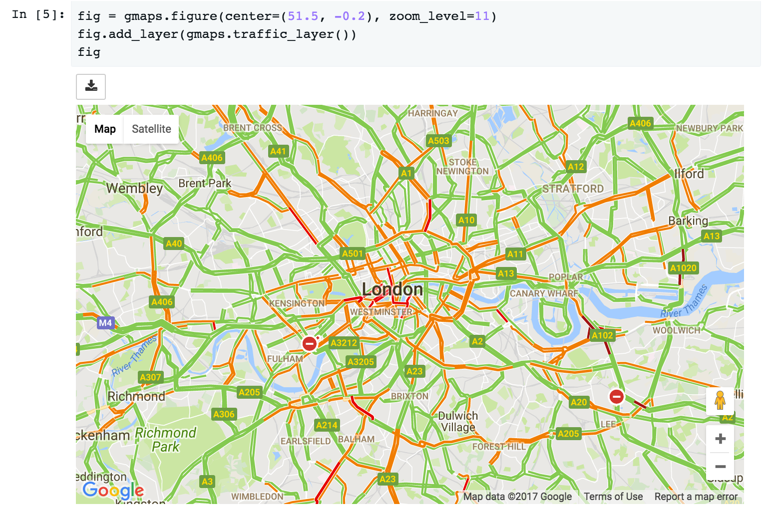
The traffic layer, available as gmaps.traffic_layer(), adds information about the current state of traffic.

Unlike the other layers, these layers do not take any user data. Thus, jupyter-gmaps will not use them to center the map. This means that, if you use these layers by themselves, you will often want to center the figure explicitly, using the center and zoom_level attributes.